Feature Engineering: Turning Raw Data into Model-Visible Signal

ML
Feature Engineering
Data Science
A practical and visual guide to numerical, categorical, temporal, text, interaction, aggregation, geospatial, missing-value, dimensionality-reduction and domain feature engineering—with simulations, Python, pipelines and leakage-safe thinking.
Author

MLStation

Published

October 1, 2026

🧭 Feature engineering is the art of changing the representation—not changing reality.

A model sees columns, numbers, categories and vectors. A human sees age, rush hour, customer loyalty, distance, seasonality, intent and history. Feature engineering builds the bridge.

A raw dataset rarely presents a prediction problem in the language most useful to a model.

A timestamp such as 2026-10-01 08:17:00 contains hour, weekday, month, rush-hour status and perhaps time since the previous event. A purchase table contains not only individual transactions but also customer frequency, recency and average basket value. Two latitude/longitude pairs contain distance. A sentence contains words, topics and semantic meaning.

Feature engineering turns those latent ideas into model-visible signal.

TipWhat you will learn
  • What a feature really is—and why representation matters
  • Numerical transformations, scaling, binning and nonlinear features
  • Categorical encoding, including high-cardinality strategies
  • Missing-value and missingness-indicator features
  • Dates, time, cyclical variables, lags and rolling windows
  • Interactions, ratios and domain-derived features
  • Aggregation and entity/history features
  • Text features: counts, TF–IDF and embeddings
  • Geospatial and distance features
  • Dimensionality reduction and learned representations
  • Feature selection versus feature engineering
  • Leakage, point-in-time correctness and train/test discipline
  • How to build reproducible feature pipelines in Python

1. What Is a Feature?

Suppose we want to predict whether a customer will buy a product.

Raw data:

birth_date   signup_date   city     purchases   spend
1985-03-12   2022-04-01    Austin   12          840

A model might learn more easily from:

age = 41
tenure_days = 1644
purchase_frequency = 12 / tenure_months
average_order_value = 840 / 12
city = one-hot encoded

The observation did not change.

The representation changed.

RAW DATA → TRANSFORM / COMBINE / EXTRACT → FEATURES → MODEL → PREDICTION

1.1 A useful definition

Definition 1 (Feature Engineering) Feature engineering is the process of creating, transforming, encoding, combining or selecting input variables so that relevant structure in the data is represented in a form a learning algorithm can use effectively.

The objective is not:

“Create as many columns as possible.”

It is:

Represent useful information with the least unnecessary distortion, leakage and complexity.

2. Why Can Feature Engineering Matter So Much?

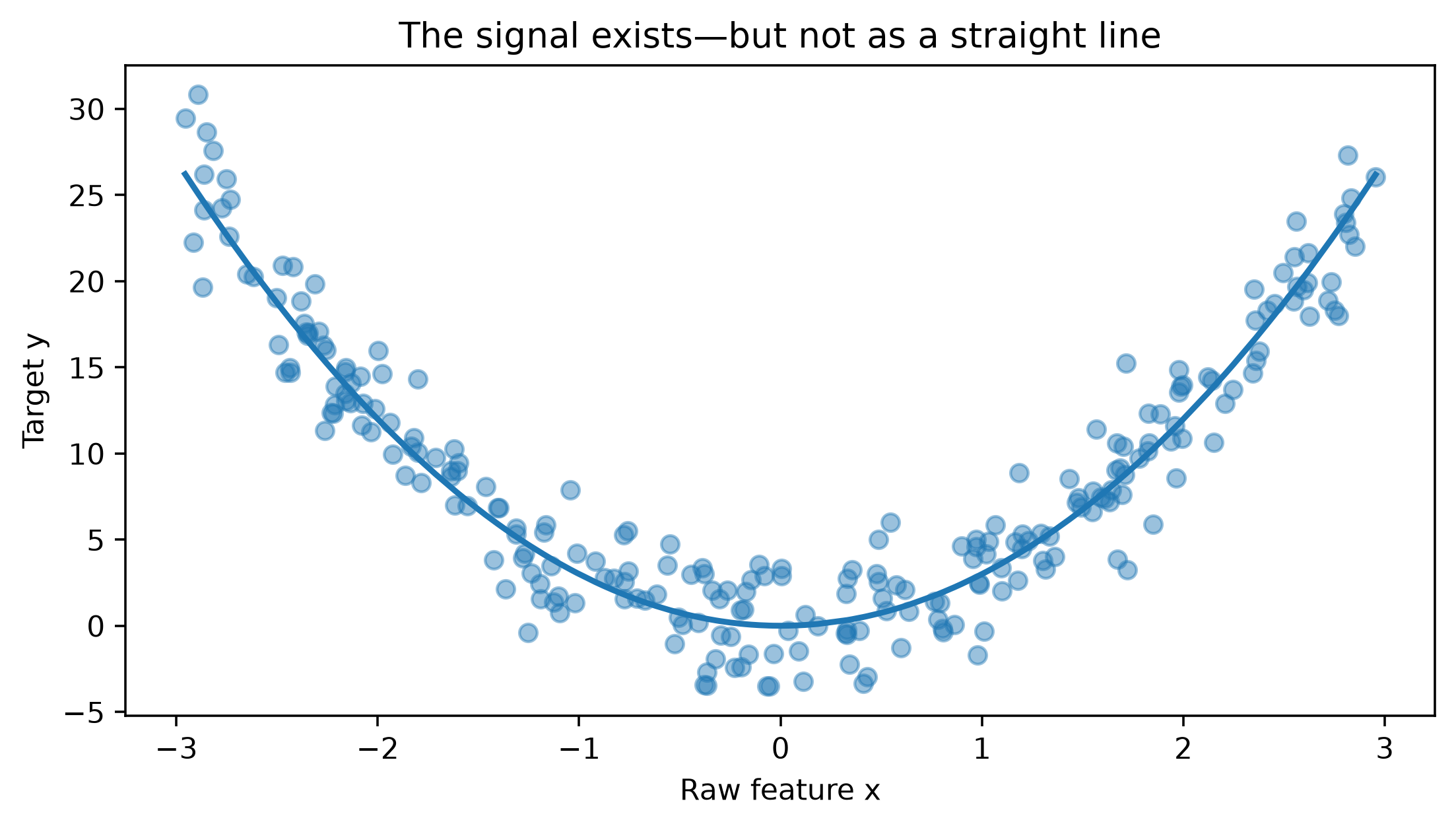
Imagine the true relationship is:

y = 3x^2 + \varepsilon.

A linear model given only x tries to learn

\hat y=\beta_0+\beta_1x.

That is the wrong vocabulary.

Give it x^2:

\hat y=\beta_0+\beta_1x+\beta_2x^2,

and suddenly a linear estimator can represent a nonlinear curve.

Show the code
import numpy as np
import pandas as pd
import matplotlib.pyplot as plt

rng = np.random.default_rng(42)
x = rng.uniform(-3, 3, 250)
y = 3 * x**2 + rng.normal(0, 2.2, len(x))

fig, ax = plt.subplots(figsize=(8, 4))
ax.scatter(x, y, alpha=.45)
order = np.argsort(x)
ax.plot(x[order], 3*x[order]**2, linewidth=2)
ax.set(xlabel="Raw feature x", ylabel="Target y",
       title="The signal exists—but not as a straight line")
plt.show()

The raw feature hides a quadratic relationship; x² exposes it.

The raw feature hides a quadratic relationship; x² exposes it.

💡 Central idea

Feature engineering and model choice interact.

  • Linear models often benefit greatly from explicit nonlinearities and interactions.
  • Distance-based methods are sensitive to scale.
  • Trees naturally learn thresholds and some interactions.
  • Neural networks can learn representations, but good inputs, normalization and domain structure can still matter.

3. A Map of Feature Engineering

🔢 Numerical

Scaling, log/power transforms, clipping, binning, splines, polynomial terms.

🏷️ Categorical

One-hot, ordinal, frequency/count, target encoding, hashing, embeddings.

❓ Missingness

Imputation, missing indicators, group-aware or model-based imputation.

📅 Time

Calendar extraction, elapsed time, cyclic encoding, lags, rolling statistics.

✖️ Interactions

Products, ratios, differences, conditional/domain interactions.

👤 Aggregation

Entity history, recency, frequency, monetary value, group summaries.

📝 Text

Counts, n-grams, TF–IDF, topics, embeddings, metadata.

🌍 Geospatial

Distance, bearing, regions, clusters, density and proximity.

🧠 Representation

PCA/SVD, learned embeddings, autoencoder/neural representations.

4. Numerical Features

Numerical features look model-ready, but their geometry and distribution may be inconvenient.

4.1 Scaling

Suppose:

age        = 42
income     = 125000
click_rate = 0.08

Their scales differ enormously.

Standardization

z=\frac{x-\mu}{\sigma}

from sklearn.preprocessing import StandardScaler

scaler = StandardScaler()
X_scaled = scaler.fit_transform(X_train[["age", "income", "click_rate"]])

Min–max scaling

x'=\frac{x-x_{\min}}{x_{\max}-x_{\min}}

Robust scaling

Median/IQR-based scaling can be preferable when extreme values are present.

NoteWhen does scaling matter most?

Usually important for:

  • k-nearest neighbors
  • k-means
  • PCA
  • SVMs
  • neural networks
  • regularized linear/logistic regression

Usually less important for ordinary decision trees and many tree ensembles.

4.2 Simulate different scales

Show the code
rng = np.random.default_rng(7)
scale_df = pd.DataFrame({
    "age": rng.normal(42, 12, 500),
    "income": rng.lognormal(11, .55, 500),
    "click_rate": rng.beta(2, 15, 500)
})

print(scale_df.agg(["mean", "std"]).round(2))
        age    income  click_rate
mean  40.46  67931.11        0.12
std   11.25  37966.13        0.08

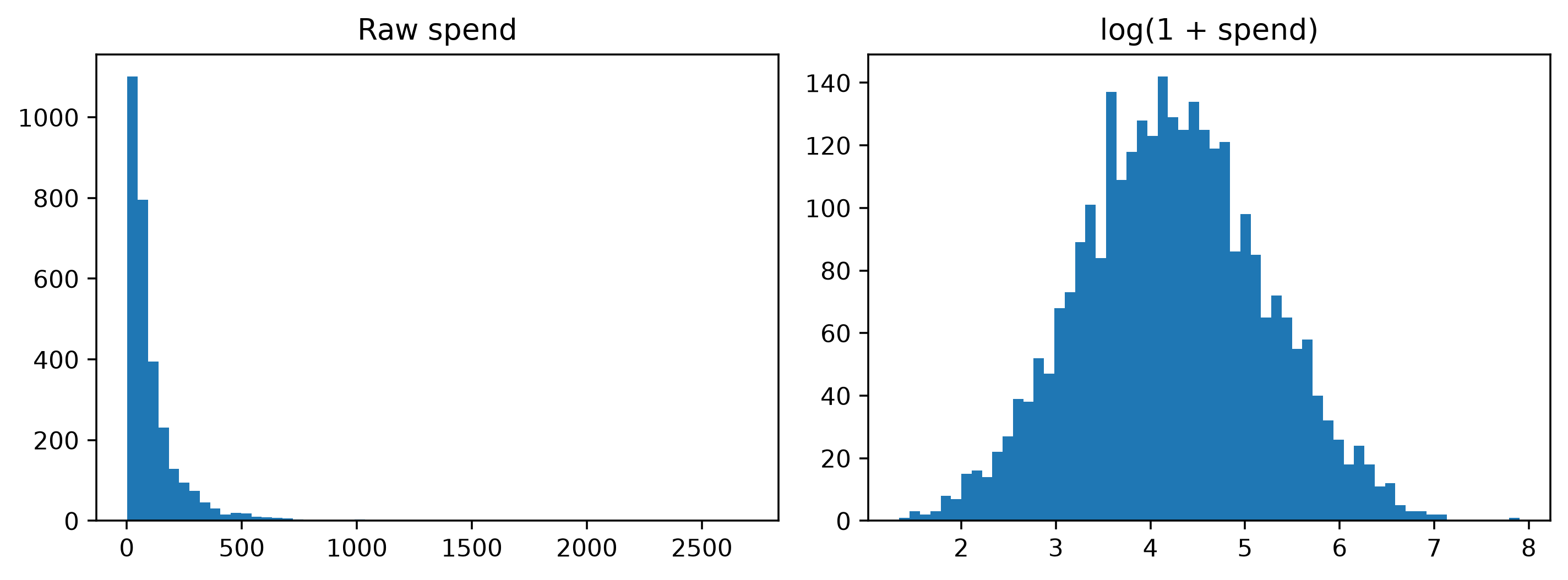
4.3 Log transforms: compress long tails

Income, transaction values, file sizes and counts often have long right tails.

Show the code
rng = np.random.default_rng(12)
spend = rng.lognormal(mean=4.2, sigma=1.0, size=3000)
log_spend = np.log1p(spend)

fig, axes = plt.subplots(1, 2, figsize=(9, 3.4))
axes[0].hist(spend, bins=60)
axes[0].set_title("Raw spend")
axes[1].hist(log_spend, bins=60)
axes[1].set_title("log(1 + spend)")
plt.tight_layout()
plt.show()

A log transform compresses the extreme right tail.

A log transform compresses the extreme right tail.

Use np.log1p(x) when zero is valid.

Other useful transforms include:

  • square root,
  • Box–Cox,
  • Yeo–Johnson,
  • quantile transforms,
  • rank transforms.

⚠️ Transformation is not a beauty contest

Do not log a variable merely to make its histogram look normal. Transform when the representation better matches the model, stabilizes scale/variance, reduces domination by extremes, or expresses a meaningful relationship.

4.4 Clipping / winsorization

Extreme values can dominate some models.

lo, hi = X_train["income"].quantile([0.01, 0.99])
X_train["income_clip"] = X_train["income"].clip(lo, hi)

Fit thresholds on training data, then reuse them.

4.5 Binning

Convert a continuous feature into intervals:

df["age_band"] = pd.cut(
    df["age"],
    bins=[0, 18, 30, 45, 65, np.inf],
    labels=["child", "young", "adult", "midlife", "senior"]
)

Binning can express thresholds, reduce sensitivity to noise, or improve interpretability—but throws away within-bin information.

5. Nonlinear Features: Polynomial Terms and Splines

5.1 Polynomial features

For features x_1 and x_2, degree-two expansion can produce:

1,\quad x_1,\quad x_2,\quad x_1^2,\quad x_1x_2,\quad x_2^2.

from sklearn.preprocessing import PolynomialFeatures

poly = PolynomialFeatures(degree=2, include_bias=False)
X_poly = poly.fit_transform(X_train[["temperature", "humidity"]])

print(poly.get_feature_names_out())

5.2 Splines

Polynomial terms are global: changing one coefficient changes the curve everywhere.

Splines build flexible smooth relationships from local basis functions.

Useful when:

  • age has a nonlinear relationship with risk,
  • demand changes smoothly with temperature,
  • response increases and then plateaus.

🌱 Think “shape,” not just “column”

age asks a model to discover what age means.

Spline features say:

“Here are several smooth basis functions from which you can build a flexible age-response curve.”

6. Categorical Features

Models cannot generally infer the meaning of strings such as:

Austin, Dallas, Houston

They need a representation.

6.1 One-hot encoding

city      Austin  Dallas  Houston
Austin       1       0       0
Houston      0       0       1
Dallas       0       1       0
from sklearn.preprocessing import OneHotEncoder

encoder = OneHotEncoder(handle_unknown="ignore")
X_city = encoder.fit_transform(X_train[["city"]])

One-hot encoding is excellent for low/moderate-cardinality nominal categories.

6.2 Ordinal encoding

Some categories have real order:

low < medium < high
from sklearn.preprocessing import OrdinalEncoder

enc = OrdinalEncoder(categories=[["low", "medium", "high"]])
df["risk_encoded"] = enc.fit_transform(df[["risk"]])

Do not impose arbitrary order on nominal categories such as city or color.

6.3 Frequency encoding

For category c:

f(c)=\frac{\#\{x_i=c\}}{n}.

Show the code
rng = np.random.default_rng(5)
cities = rng.choice(
    ["Austin", "Dallas", "Houston", "El Paso", "Other"],
    1000, p=[.25, .22, .25, .10, .18]
)
cat_df = pd.DataFrame({"city": cities})

freq = cat_df["city"].value_counts(normalize=True)
cat_df["city_frequency"] = cat_df["city"].map(freq)

print(cat_df.head())
      city  city_frequency
0  El Paso           0.100
1  El Paso           0.100
2  Houston           0.242
3   Dallas           0.214
4   Austin           0.267

Useful for high-cardinality categories, but it loses category identity: two equally frequent categories become indistinguishable.

6.4 Target / mean encoding

For category c:

TE(c)\approx E[Y\mid X=c].

This can be powerful for high-cardinality features such as:

  • product ID,
  • ZIP code,
  • advertiser,
  • merchant,
  • publisher.

But it is dangerous.

🚨 Leakage alert: target encoding

If you calculate a category’s target mean using the same row’s target, information from y leaks into X.

Training features should be generated out-of-fold or with an encoder/pipeline that handles the training procedure correctly. Validation/test encodings must be learned from training data only.

6.5 Other categorical strategies

  • binary encoding,
  • hashing trick,
  • count encoding,
  • rare-category grouping,
  • learned entity embeddings.

The best representation depends on cardinality, model family, dataset size and whether new categories appear after deployment.

7. Missing Values Are Sometimes Information

Suppose income is missing.

The naive interpretation is:

“We do not know income.”

But perhaps income is missing because:

  • the customer declined to provide it,
  • a legacy system did not collect it,
  • a certain acquisition channel skips the field.

Then missingness itself may be predictive.

7.1 Simulate informative missingness

Show the code
rng = np.random.default_rng(17)
n = 2500

income = rng.lognormal(11, .45, n)
premium = (income > np.quantile(income, .7)).astype(int)

# Higher-income users are more likely to omit income in this toy example.
missing_prob = .08 + .35 * premium
missing = rng.random(n) < missing_prob

missing_df = pd.DataFrame({
    "income": income,
    "premium": premium
})
missing_df.loc[missing, "income"] = np.nan
missing_df["income_missing"] = missing_df["income"].isna().astype(int)

print(missing_df.groupby("income_missing")["premium"].mean())
income_missing
0    0.201178
1    0.735931
Name: premium, dtype: float64

7.2 Imputation + indicator

from sklearn.impute import SimpleImputer

imp = SimpleImputer(strategy="median", add_indicator=True)
X_imp = imp.fit_transform(X_train[["income", "age"]])

Common approaches:

  • mean/median imputation,
  • most-frequent category,
  • explicit "Missing" category,
  • missingness indicator,
  • KNN/model-based imputation,
  • domain-specific rules.
WarningMissing-value engineering requires causal humility

A missingness pattern that predicts well today can disappear when the upstream data-collection system changes.

8. Date and Time Features

A timestamp is a compressed package of potential features.

ts = pd.to_datetime(df["timestamp"])

df["hour"] = ts.dt.hour
df["weekday"] = ts.dt.dayofweek
df["month"] = ts.dt.month
df["is_weekend"] = (ts.dt.dayofweek >= 5).astype(int)
df["quarter"] = ts.dt.quarter

Other useful features:

  • day of month,
  • week of year,
  • holiday indicator,
  • business day,
  • season,
  • days since signup,
  • time since last event,
  • time until deadline.

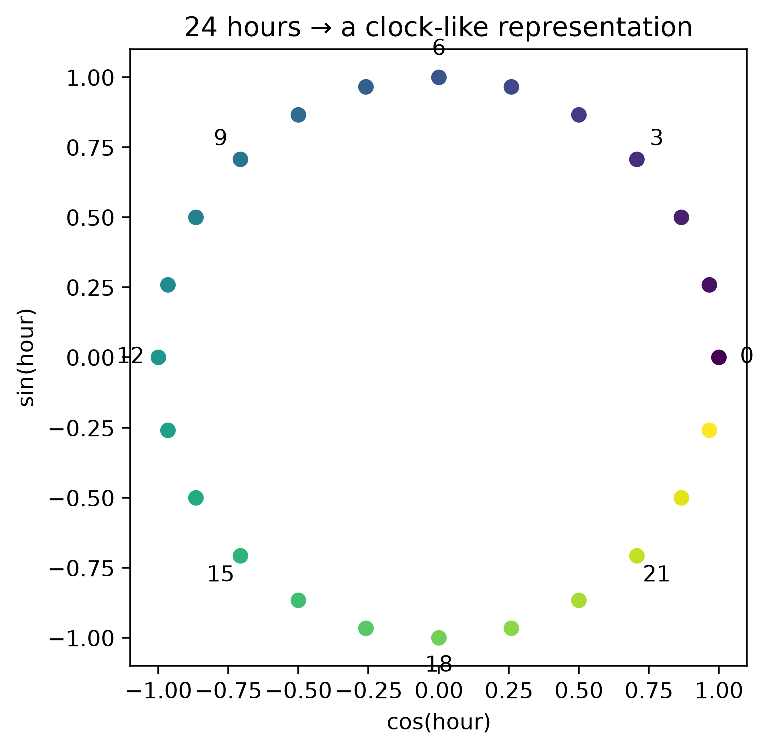
8.1 Cyclical encoding

Hour 23 and hour 0 are neighbors in reality.

Numerically:

|23-0|=23.

That representation is misleading.

Map the cycle onto a circle:

x_{\sin}=\sin\left(2\pi\frac{x}{P}\right),

x_{\cos}=\cos\left(2\pi\frac{x}{P}\right).

Show the code
hours = np.arange(24)
hour_sin = np.sin(2*np.pi*hours/24)
hour_cos = np.cos(2*np.pi*hours/24)

fig, ax = plt.subplots(figsize=(5,5))
sc = ax.scatter(hour_cos, hour_sin, c=hours)
for h, x0, y0 in zip(hours, hour_cos, hour_sin):
    if h % 3 == 0:
        ax.text(x0*1.10, y0*1.10, str(h), ha="center", va="center")
ax.set(xlabel="cos(hour)", ylabel="sin(hour)", title="24 hours → a clock-like representation")
ax.set_aspect("equal")
plt.show()

Hours wrap around a circle: midnight becomes adjacent to 23:00 and 01:00.

Hours wrap around a circle: midnight becomes adjacent to 23:00 and 01:00.
df["hour_sin"] = np.sin(2*np.pi*df["hour"]/24)
df["hour_cos"] = np.cos(2*np.pi*df["hour"]/24)

9. Time-Series Features: Lags and Rolling Windows

For ordered data, the past is often the most useful feature source.

9.1 Lag features

x_t^{(1)}=y_{t-1}

df["sales_lag_1"] = df["sales"].shift(1)
df["sales_lag_7"] = df["sales"].shift(7)

9.2 Rolling statistics

df["sales_mean_7"] = (
    df["sales"]
      .shift(1)
      .rolling(7)
      .mean()
)

Notice the shift(1).

Why?

At prediction time for day t, today’s target y_t is not yet known.

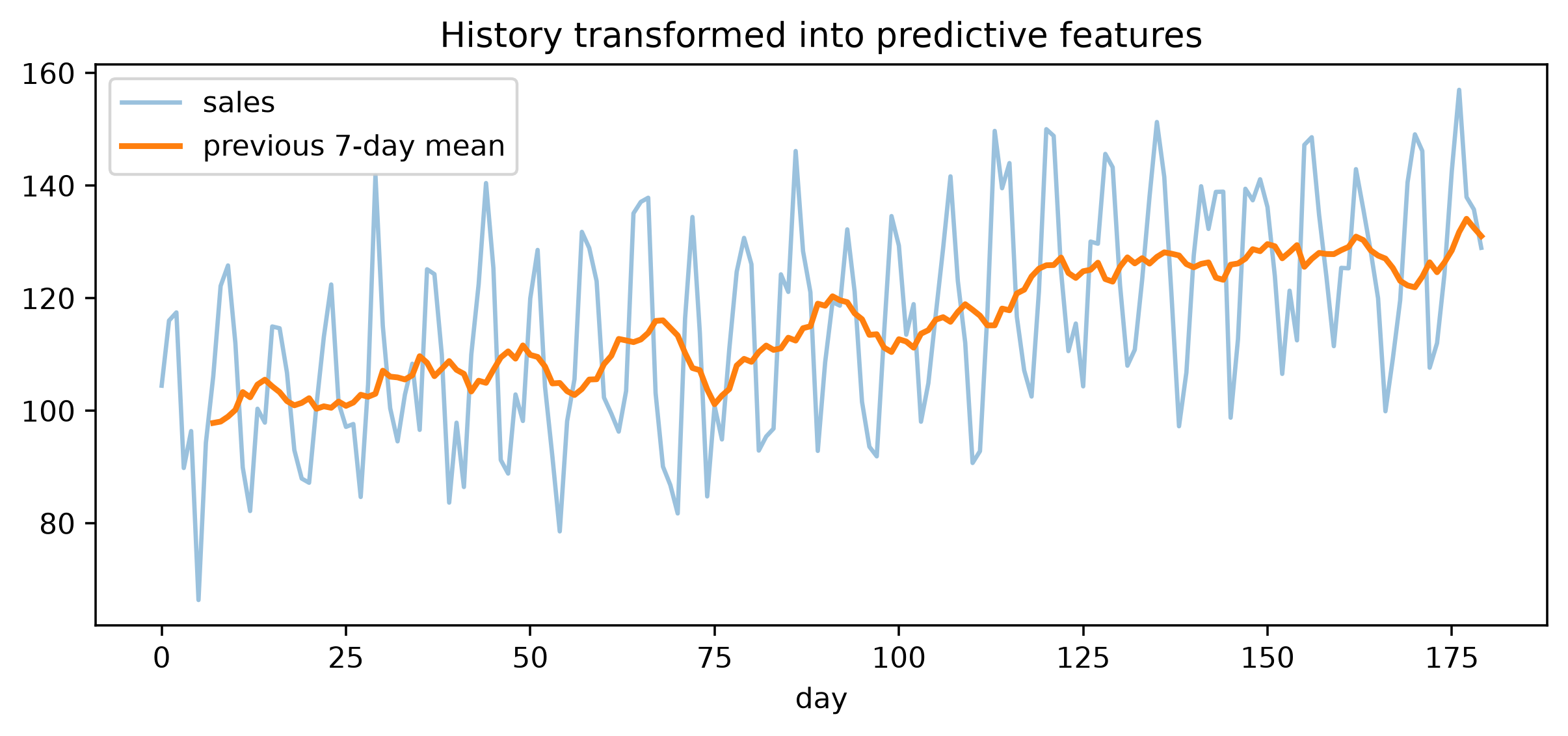
9.3 Simulate a seasonal series

Show the code
rng = np.random.default_rng(23)
n = 180
t = np.arange(n)

sales = (
    100
    + .18*t
    + 18*np.sin(2*np.pi*t/7)
    + rng.normal(0, 8, n)
)

ts_df = pd.DataFrame({"day": t, "sales": sales})
ts_df["lag_1"] = ts_df["sales"].shift(1)
ts_df["lag_7"] = ts_df["sales"].shift(7)
ts_df["rolling_7"] = ts_df["sales"].shift(1).rolling(7).mean()

fig, ax = plt.subplots(figsize=(9,3.5))
ax.plot(ts_df["day"], ts_df["sales"], alpha=.45, label="sales")
ax.plot(ts_df["day"], ts_df["rolling_7"], linewidth=2, label="previous 7-day mean")
ax.legend()
ax.set(title="History transformed into predictive features", xlabel="day")
plt.show()

🚨 Point-in-time correctness

For prediction at time t, every feature must be constructible using information available at or before the prediction cutoff.

A perfectly predictive feature from tomorrow is not brilliant feature engineering. It is leakage.

10. Interaction Features: When “Together” Matters

Sometimes x_1 matters only in the presence of x_2.

Examples:

temperature × humidity
income / household_size
price × discount
age × medication
hour × working_day

10.1 Simulate a pure interaction

Let:

y=4x_1x_2+\varepsilon.

Individually, x_1 and x_2 may look weak. Their product contains the signal.

Show the code
rng = np.random.default_rng(29)
n = 1500
x1 = rng.normal(size=n)
x2 = rng.normal(size=n)
y = 4*x1*x2 + rng.normal(0, 1, n)

interaction_df = pd.DataFrame({
    "x1": x1,
    "x2": x2,
    "x1_x2": x1*x2,
    "y": y
})

print(interaction_df.corr(numeric_only=True)["y"].round(3))
x1      -0.003
x2       0.049
x1_x2    0.967
y        1.000
Name: y, dtype: float64
df["temp_humidity"] = df["temperature"] * df["humidity"]
df["spend_per_visit"] = df["total_spend"] / df["visits"].clip(lower=1)

10.2 Ratios and differences

Often domain relationships matter more than raw values:

  • BMI = weight / height²,
  • price per square foot,
  • debt-to-income ratio,
  • current balance − previous balance,
  • actual − expected,
  • clicks / impressions.

⚠️ Ratios can explode

If the denominator is near zero, a ratio becomes unstable. Handle zero explicitly and inspect the resulting distribution.

11. Aggregation Features: Turn Events into Behavior

Suppose your raw table contains transactions:

customer   date        amount
A          Jan 01      20
A          Jan 04      80
A          Jan 18      35
B          Jan 03      15

For customer-level prediction, useful features might be:

number_of_orders
total_spend
average_order_value
maximum_order
days_since_last_order
orders_last_30_days
spend_last_90_days

11.1 Simulate transactions

Show the code
rng = np.random.default_rng(31)
n_customers = 250
n_tx = 5000

transactions = pd.DataFrame({
    "customer_id": rng.integers(0, n_customers, n_tx),
    "amount": rng.lognormal(3.3, .7, n_tx),
    "day": rng.integers(0, 365, n_tx)
})

customer_features = (
    transactions.groupby("customer_id")
    .agg(
        order_count=("amount", "size"),
        total_spend=("amount", "sum"),
        avg_order_value=("amount", "mean"),
        max_order_value=("amount", "max"),
        last_purchase_day=("day", "max"),
    )
)

customer_features["recency"] = 365 - customer_features["last_purchase_day"]
print(customer_features.head())
             order_count  total_spend  avg_order_value  max_order_value  \
customer_id                                                               
0                     24   787.439330        32.809972        87.982895   
1                     22   739.587347        33.617607       122.219902   
2                     17   526.823425        30.989613        88.390128   
3                     21   771.301799        36.728657        83.150738   
4                     21   684.098490        32.576119       104.837612   

             last_purchase_day  recency  
customer_id                              
0                          340       25  
1                          359        6  
2                          327       38  
3                          362        3  
4                          363        2  

This is the basis of RFM thinking:

  • Recency,
  • Frequency,
  • Monetary value.

11.2 Group statistics

A row can be compared with its peer group:

df["category_avg_price"] = (
    df.groupby("category")["price"].transform("mean")
)

df["price_vs_category"] = (
    df["price"] / df["category_avg_price"]
)

But when the target or future observations are involved, group features must be built carefully using only permissible information.

12. Text Feature Engineering

Text begins as unstructured strings:

"The battery life is excellent."

A model needs a numerical representation.

12.1 Bag of words

Represent documents by token counts.

12.2 N-grams

Unigrams:

not, very, good

Bigrams:

not very, very good

N-grams preserve limited local word order.

12.3 TF–IDF

TF–IDF increases weight for terms important to a document but less common across the collection.

from sklearn.feature_extraction.text import TfidfVectorizer

tfidf = TfidfVectorizer(
    ngram_range=(1, 2),
    min_df=2,
    max_features=20_000
)

X_text = tfidf.fit_transform(train_text)

12.4 Simulate text metadata

Even before semantic modeling, useful features can include:

text_df["char_count"] = text_df["text"].str.len()
text_df["word_count"] = text_df["text"].str.split().str.len()
text_df["question_marks"] = text_df["text"].str.count(r"\?")
text_df["exclamation_marks"] = text_df["text"].str.count("!")

12.5 Embeddings

Modern embedding models map text to dense vectors:

\text{text}\longrightarrow \mathbf{e}\in\mathbb{R}^d.

Semantically similar text can be nearby in embedding space.

"refund my payment" ─┐
                     ├── nearby vectors
"money back please" ─┘

Embeddings are learned feature representations. They extend feature engineering beyond manually designed columns.

13. Geospatial Features

Raw coordinates:

latitude, longitude

often become much more meaningful when converted into relationships.

Useful features include:

  • distance to store,
  • distance to city center,
  • nearest facility,
  • number of facilities within radius,
  • region/ZIP/geohash,
  • local density,
  • bearing,
  • travel-time proxy.

13.1 Haversine distance

For points on Earth:

#| code-fold: true
#| code-summary: "Show geospatial simulation code"

import numpy as np
import pandas as pd

def haversine_km(lat1, lon1, lat2, lon2):
    """Great-circle distance between coordinates in kilometers."""
    R = 6371.0

    lat1 = np.radians(lat1)
    lon1 = np.radians(lon1)
    lat2 = np.radians(lat2)
    lon2 = np.radians(lon2)

    dlat = lat2 - lat1
    dlon = lon2 - lon1

    a = (
        np.sin(dlat / 2)**2
        + np.cos(lat1)
        * np.cos(lat2)
        * np.sin(dlon / 2)**2
    )

    return 2 * R * np.arcsin(np.sqrt(a))


## 13.2 Simulate customer locations around Austin
rng = np.random.default_rng(37)

geo = pd.DataFrame({
    "lat": 30.27 + rng.normal(0, 0.08, 800),
    "lon": -97.74 + rng.normal(0, 0.08, 800)
})

# Example store location
store_lat = 30.2672
store_lon = -97.7431

geo["distance_to_store_km"] = haversine_km(
    geo["lat"],
    geo["lon"],
    store_lat,
    store_lon
)

print(
    geo["distance_to_store_km"]
    .describe()
    .round(2)
)

Coordinates tell the model where. Distance features can tell it how far from something relevant.

14. Domain Features: Where Expertise Becomes Data

Some of the highest-value features cannot be discovered from a generic preprocessing recipe.

Examples:

Finance

  • debt-to-income,
  • utilization ratio,
  • payment-to-balance,
  • days delinquent.

E-commerce

  • cart value,
  • days since last purchase,
  • repeat-purchase rate,
  • discount sensitivity.

Cybersecurity

  • failed logins in previous hour,
  • number of unique destinations,
  • deviation from user’s normal behavior,
  • rare process/network combinations.

Healthcare

  • age at event,
  • change from baseline,
  • dosage per body weight,
  • time since previous visit.

Physics / engineering

  • normalized residual,
  • signal-to-noise ratio,
  • invariant combinations,
  • dimensionless quantities.

🧠 Domain knowledge is a representation engine

A domain expert often knows that two raw measurements should become a ratio, difference, rate, residual, normalized quantity or historical deviation.

That knowledge can make a simple model remarkably strong.

15. Feature Engineering for Images, Audio and Signals

Feature engineering is not restricted to tables.

Images

Classical engineered features include:

  • edges,
  • corners,
  • color histograms,
  • HOG,
  • SIFT-like local descriptors,
  • texture measures.

Modern deep learning often learns representations directly through convolutional or vision-transformer layers.

Audio / signals

Common engineered representations include:

  • frequency-domain features,
  • FFT coefficients,
  • spectral power,
  • MFCCs,
  • rolling energy,
  • peaks,
  • zero-crossing rate,
  • wavelet features.

The same principle survives:

RAW SIGNAL → REPRESENTATION → USEFUL STRUCTURE → MODEL

16. Dimensionality Reduction as Feature Construction

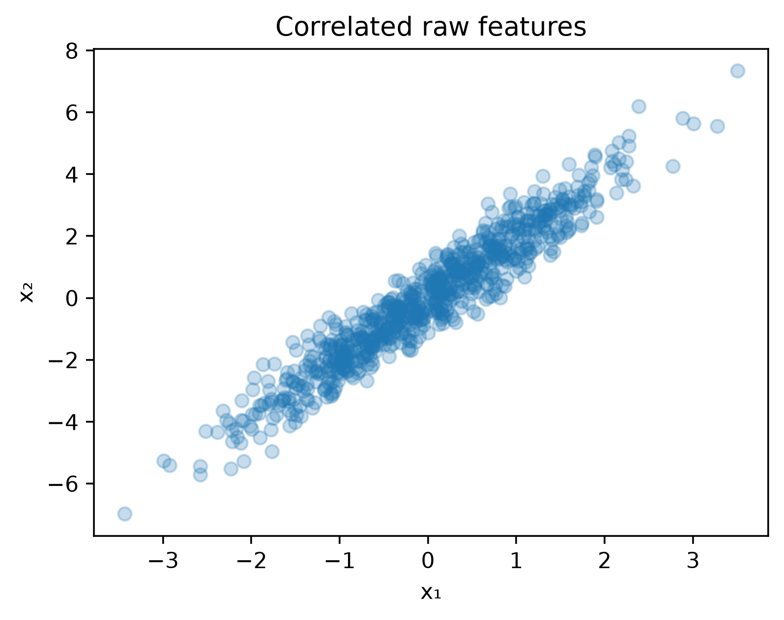
Sometimes feature engineering means replacing many correlated variables with a smaller representation.

16.1 PCA

Principal Component Analysis constructs:

z_1=w_{11}x_1+w_{12}x_2+\cdots+w_{1p}x_p

so that early components capture large directions of variance.

Show the code
from sklearn.decomposition import PCA

rng = np.random.default_rng(41)
x = rng.normal(size=800)
X2 = np.c_[x + rng.normal(0,.25,800),
           2*x + rng.normal(0,.35,800)]

pca = PCA(n_components=2)
Z = pca.fit_transform(X2)

fig, ax = plt.subplots(figsize=(5.5,4))
ax.scatter(X2[:,0], X2[:,1], alpha=.25)
ax.set(title="Correlated raw features", xlabel="x₁", ylabel="x₂")
plt.show()

print("Explained variance ratio:", pca.explained_variance_ratio_.round(3))

Correlated raw features can be rotated into principal-component coordinates.

Correlated raw features can be rotated into principal-component coordinates.
Explained variance ratio: [0.987 0.013]

Related approaches:

  • PCA,
  • truncated SVD,
  • NMF,
  • autoencoders,
  • learned embeddings.
NoteFeature extraction vs. feature selection

Extraction creates a new representation, such as principal components.

Selection keeps a subset of existing features.

17. Feature Selection

More features are not automatically better.

Irrelevant or redundant features can:

  • increase variance,
  • slow training,
  • increase storage/serving cost,
  • complicate interpretation,
  • increase leakage risk.

17.1 Filter methods

Independent of the final model:

  • variance threshold,
  • correlation filtering,
  • mutual information,
  • univariate statistical tests.

17.2 Wrapper methods

Evaluate subsets using a model:

  • recursive feature elimination,
  • sequential selection.

17.3 Embedded methods

Selection occurs during model fitting:

  • L1 regularization,
  • tree-based importance,
  • regularized models.

⚠️ Importance is not usefulness in isolation

Correlated features can share or substitute for predictive information. Feature importance depends on the model, data distribution and importance method.

18. The Most Dangerous Feature: Leakage

Suppose you predict whether a loan will default.

You create:

days_since_last_collection_call

but collection calls occur after default trouble begins.

The model performs spectacularly.

It has learned the future.

18.1 Three common leakage families

Target leakage

The feature directly or indirectly contains the target.

Train/test contamination

Scaler, imputer, encoder or selector is fitted using validation/test data.

Temporal leakage

The feature uses information unavailable at prediction time.

🚨 The Feature Availability Test

For every feature, ask:

At the exact moment this prediction would be made in production, could I compute this feature using only information legitimately available then?

If the answer is no, the feature does not belong in the model.

19. Fit on Train, Transform Everywhere

This pattern is essential.

Wrong:

# DON'T
X_scaled = StandardScaler().fit_transform(X)
X_train, X_test = train_test_split(X_scaled)

Correct:

X_train, X_test, y_train, y_test = train_test_split(
    X, y, test_size=0.2, random_state=42
)

scaler = StandardScaler()
X_train_scaled = scaler.fit_transform(X_train)
X_test_scaled = scaler.transform(X_test)

Better still: use a pipeline.

20. Production-Friendly Feature Engineering with Pipelines

Suppose we have:

  • numerical columns,
  • categorical columns,
  • missing values.
from sklearn.compose import ColumnTransformer
from sklearn.impute import SimpleImputer
from sklearn.pipeline import Pipeline
from sklearn.preprocessing import OneHotEncoder, StandardScaler
from sklearn.linear_model import LogisticRegression

numeric_features = ["age", "income", "tenure_days"]
categorical_features = ["city", "device"]

numeric_pipe = Pipeline([
    ("impute", SimpleImputer(strategy="median", add_indicator=True)),
    ("scale", StandardScaler()),
])

categorical_pipe = Pipeline([
    ("impute", SimpleImputer(strategy="most_frequent")),
    ("onehot", OneHotEncoder(handle_unknown="ignore")),
])

features = ColumnTransformer([
    ("num", numeric_pipe, numeric_features),
    ("cat", categorical_pipe, categorical_features),
])

model = Pipeline([
    ("features", features),
    ("classifier", LogisticRegression(max_iter=1000)),
])

model.fit(X_train, y_train)
pred = model.predict_proba(X_test)[:, 1]

Why is this beautiful?

TRAIN
raw rows
   ↓
fit imputer
   ↓
fit scaler / encoder
   ↓
fit model

TEST / PRODUCTION
raw rows
   ↓
reuse SAME learned transformations
   ↓
reuse SAME model

The feature logic becomes part of the model artifact.

21. A Complete Simulated Example: Customer Churn

Now combine several ideas.

21.1 Simulate raw customer data

Show the code
rng = np.random.default_rng(101)
n = 4000

customers = pd.DataFrame({
    "age": rng.integers(18, 80, n),
    "monthly_spend": rng.lognormal(3.7, .55, n),
    "support_calls_90d": rng.poisson(1.5, n),
    "tenure_months": rng.integers(1, 96, n),
    "plan": rng.choice(["basic", "plus", "premium"], n, p=[.5,.35,.15]),
    "last_login_days": rng.exponential(8, n),
})

logit = (
    -2.2
    + .055 * customers["last_login_days"]
    + .20 * customers["support_calls_90d"]
    - .018 * customers["tenure_months"]
    + .45 * (customers["plan"] == "basic")
)

p = 1/(1+np.exp(-logit))
customers["churn"] = rng.binomial(1, p)

print(customers.head())
print("Churn rate:", customers["churn"].mean().round(3))
   age  monthly_spend  support_calls_90d  tenure_months   plan  \
0   37      64.474255                  0             86  basic   
1   76      22.955691                  0             37   plus   
2   61      46.536471                  4             95   plus   
3   40      46.711199                  3             33   plus   
4   26      76.409626                  2             94   plus   

   last_login_days  churn  
0        17.357256      0  
1         2.943766      0  
2        16.659506      0  
3         3.554885      0  
4         6.779185      0  
Churn rate: 0.125

21.2 Engineer meaningful features

customers["spend_per_tenure"] = (
    customers["monthly_spend"]
    / customers["tenure_months"].clip(lower=1)
)

customers["is_inactive_14d"] = (
    customers["last_login_days"] >= 14
).astype(int)

customers["support_pressure"] = (
    customers["support_calls_90d"]
    / np.sqrt(customers["tenure_months"])
)

customers["log_monthly_spend"] = np.log1p(
    customers["monthly_spend"]
)

Each feature expresses a hypothesis:

spend_per_tenure
→ Is spending unusually high relative to relationship length?

is_inactive_14d
→ Has engagement crossed a meaningful inactivity threshold?

support_pressure
→ Is support demand high relative to customer maturity?

log_monthly_spend
→ Compress extreme spending differences.

That is the mindset.

22. How Do We Know a Feature Is Good?

A feature is not good because it sounds clever.

Evaluate it.

22.1 Ablation

Compare:

Model A → baseline features
Model B → baseline + new feature family

Use the same validation protocol.

22.2 Stability

Ask whether the feature:

  • works across folds,
  • works across time,
  • works across important segments,
  • remains available in production,
  • has a stable distribution.

22.3 Cost

A feature can improve AUC by 0.001 and still be a bad production feature if it requires:

  • an expensive external API,
  • a 30-minute aggregation,
  • fragile joins,
  • unavailable real-time data.

Feature quality is multi-dimensional:

\text{Value} \approx \frac{\text{predictive gain}\times\text{stability}\times\text{interpretability}} {\text{latency}+\text{cost}+\text{complexity}+\text{leakage risk}}.

This is a mental model—not a literal universal formula.

23. Feature Engineering by Model Family

Model family Feature-engineering considerations
Linear / Logistic Scaling, nonlinear basis terms and interactions can matter greatly
kNN / k-means Scaling and meaningful distance geometry are critical
SVM Scaling is usually important; kernels alter representation
Trees / Random Forest Scaling usually unnecessary; thresholds/interactions often learned naturally
Gradient Boosting Strong on tabular nonlinearities; domain/history features still valuable
Neural Networks Often learn representations; normalization and structured inputs still matter
Time-series models Lags, rolling windows, calendar and point-in-time correctness
NLP linear models TF–IDF/n-grams often strong baselines
Modern NLP pretrained embeddings/transformer representations

24. What About Automated Feature Engineering?

Feature generation can be automated:

  • polynomial expansion,
  • interaction search,
  • aggregation frameworks,
  • feature stores,
  • representation learning,
  • AutoML preprocessing.

But automation does not eliminate the hardest questions:

What information is legitimate?
What existed at prediction time?
What does the business process mean?
Will this feature exist in production?
Will its definition remain stable?

Those are reasoning problems.

25. Feature Stores and Production Consistency

At scale, organizations may maintain reusable feature definitions so training and serving compute the same concept.

A feature definition needs more than a name:

feature: orders_last_30d
entity: customer_id
event time: order_timestamp
window: previous 30 days
cutoff: prediction_timestamp
null policy: 0
version: v3
owner: retention_team

This is feature engineering becoming data-system engineering.

26. A Practical Checklist

Before creating a feature:

  • What real-world concept does it represent?
  • Why should it relate to the target?
  • Is the relationship linear, nonlinear, periodic or conditional?
  • Is the value available at prediction time?

Before fitting:

  • Which transformations must be learned from training data?
  • Are categories unseen in validation/production handled?
  • Are missing values handled?
  • Are extreme values plausible?

Before shipping:

  • Can the feature be computed reliably?
  • Is offline computation identical to online computation?
  • Is latency acceptable?
  • Can its distribution be monitored?
  • Is the definition/version documented?

27. The Feature Engineer’s Ladder

Level 1  CLEAN
         types, missingness, impossible values
            ↓
Level 2  REPRESENT
         scale, encode, transform
            ↓
Level 3  EXTRACT
         dates, text, geography, signal structure
            ↓
Level 4  COMBINE
         ratios, differences, interactions
            ↓
Level 5  REMEMBER
         lags, rolling windows, entity history
            ↓
Level 6  LEARN
         PCA, embeddings, representation learning
            ↓
Level 7  VALIDATE
         ablation, CV, temporal validation, stability
            ↓
Level 8  PRODUCTIONIZE
         pipelines, point-in-time correctness, monitoring

28. Final Perspective

Feature engineering is where three kinds of knowledge meet:

\boxed{ \text{Data Understanding} + \text{Domain Knowledge} + \text{Model Understanding} }

A beginner often asks:

“Which transformation should I use?”

A stronger question is:

“What structure exists in the real problem, and what representation would make that structure accessible to this model without leaking unavailable information?”

That question scales from a two-column regression problem to recommendation systems, fraud detection, forecasting and modern AI.

✨ The model learns from the world you show it.

Feature engineering decides how the world is shown.

Summary

  • Feature engineering changes representation, not the underlying observation.
  • Numerical features may need scaling, transforms, clipping, bins, splines or polynomial terms.
  • Categorical variables can use one-hot, ordinal, frequency, target, hashing or learned representations.
  • Missingness can itself contain signal.
  • Dates should often become calendar, elapsed-time and cyclic features.
  • Time-series features require lags, rolling summaries and strict point-in-time correctness.
  • Interactions, ratios and domain-derived quantities can expose relationships raw columns hide.
  • Aggregations turn event history into entity behavior.
  • Text can become counts, TF–IDF or learned embeddings.
  • Geography becomes more useful through distance, region and proximity features.
  • PCA and embeddings construct lower-dimensional or learned representations.
  • Feature selection controls redundancy, complexity and cost.
  • Leakage can make invalid features appear spectacular.
  • Pipelines keep training and inference transformations consistent.
  • The value of a feature must be demonstrated by validation, stability and operational usefulness.

Further reading

  • scikit-learn preprocessing documentation: scaling, encoding, polynomial features, splines and other transformers.
  • scikit-learn time-related feature-engineering example for cyclical and periodic representations.
  • pandas User Guide for missing data, categoricals, grouping, windowing and time-series manipulation.
Back to top