Model Evaluation: How Do We Know the Model Is Actually Good?
ML
Evaluation
Data Science
A rigorous but intuitive guide to validation design, regression and classification metrics, thresholds, calibration, cross-validation, uncertainty, leakage and business-aware model evaluation.
Author
MLStation
Published
October 1, 2026
🧪 Training asks: “Can the model learn?” Evaluation asks: “Can I trust what it learned?”
A model can achieve 99% accuracy and be useless. It can have excellent ROC-AUC and produce poor probabilities. It can dominate random cross-validation and fail next month. Evaluation is therefore a design problem, not merely a metric calculation.
1. The Fundamental Rule: Evaluate Unseen Data
If model parameters are learned from \mathcal D_{\text{train}}, performance must be estimated on data not used to fit those parameters.
ALL DATA
   │
   ├── TRAIN ── learn parameters
   │
   ├── VALIDATION ── choose/tune
   │
   └── TEST ── final unbiased-ish assessment
WarningThe test set is not a development dashboard
If you repeatedly inspect test performance and change the model, the test set becomes part of model development.
2. Simulate a Realistic Binary Classification Problem
Show simulated churn-data code
import numpy as np, pandas as pdimport matplotlib.pyplot as pltfrom sklearn.datasets import make_classificationfrom sklearn.model_selection import train_test_splitX,y=make_classification( n_samples=6000,n_features=12,n_informative=6, n_redundant=2,weights=[.86,.14], class_sep=1.0,flip_y=.025,random_state=42)X_train,X_test,y_train,y_test=train_test_split( X,y,test_size=.25,stratify=y,random_state=42)
3. Always Build a Baseline
For imbalanced classification, predicting the majority class may yield high accuracy.
Show the code
from sklearn.dummy import DummyClassifierdummy=DummyClassifier(strategy="prior")dummy.fit(X_train,y_train)print("Dummy accuracy:",dummy.score(X_test,y_test))
Dummy accuracy: 0.852
Your model should beat a meaningful baseline—not merely produce a large-looking number.
4. The Confusion Matrix
For binary classification:
Predicted −
Predicted +
Actual −
TN
FP
Actual +
FN
TP
From these four counts, many recurring metrics emerge.
5. Accuracy
\text{Accuracy}=\frac{TP+TN}{TP+TN+FP+FN}.
Useful when classes and error costs are reasonably balanced.
Dangerous when the positive class is rare or errors have asymmetric cost.
6. Precision and Recall
\text{Precision}=\frac{TP}{TP+FP}
asks:
Of the cases we flagged, how many were truly positive?
\text{Recall}=\frac{TP}{TP+FN}
asks:
Of all true positives, how many did we catch?
Use-case intuition
Fraud investigation with limited analysts: precision matters.
Cancer screening where missing a case is costly: recall can matter strongly.
Neither metric should be selected without the decision context.
from sklearn.linear_model import LogisticRegressionfrom sklearn.metrics import precision_score, recall_score, f1_scoreclf=LogisticRegression(max_iter=1000).fit(X_train,y_train)prob=clf.predict_proba(X_test)[:,1]rows=[]for t in np.linspace(.05,.95,19): pred=(prob>=t).astype(int) rows.append({"threshold":t,"precision":precision_score(y_test,pred,zero_division=0),"recall":recall_score(y_test,pred,zero_division=0),"f1":f1_score(y_test,pred,zero_division=0) })threshold_df=pd.DataFrame(rows)
Show the code
import plotly.express as pxlong=threshold_df.melt("threshold",var_name="metric",value_name="score")fig=px.line(long,x="threshold",y="score",color="metric", markers=True,title="Threshold changes the operating point")fig.show()
Model selection and decision selection are different
First learn a scoring/ranking model. Then choose an operating threshold based on costs, capacity, risk and product objectives.
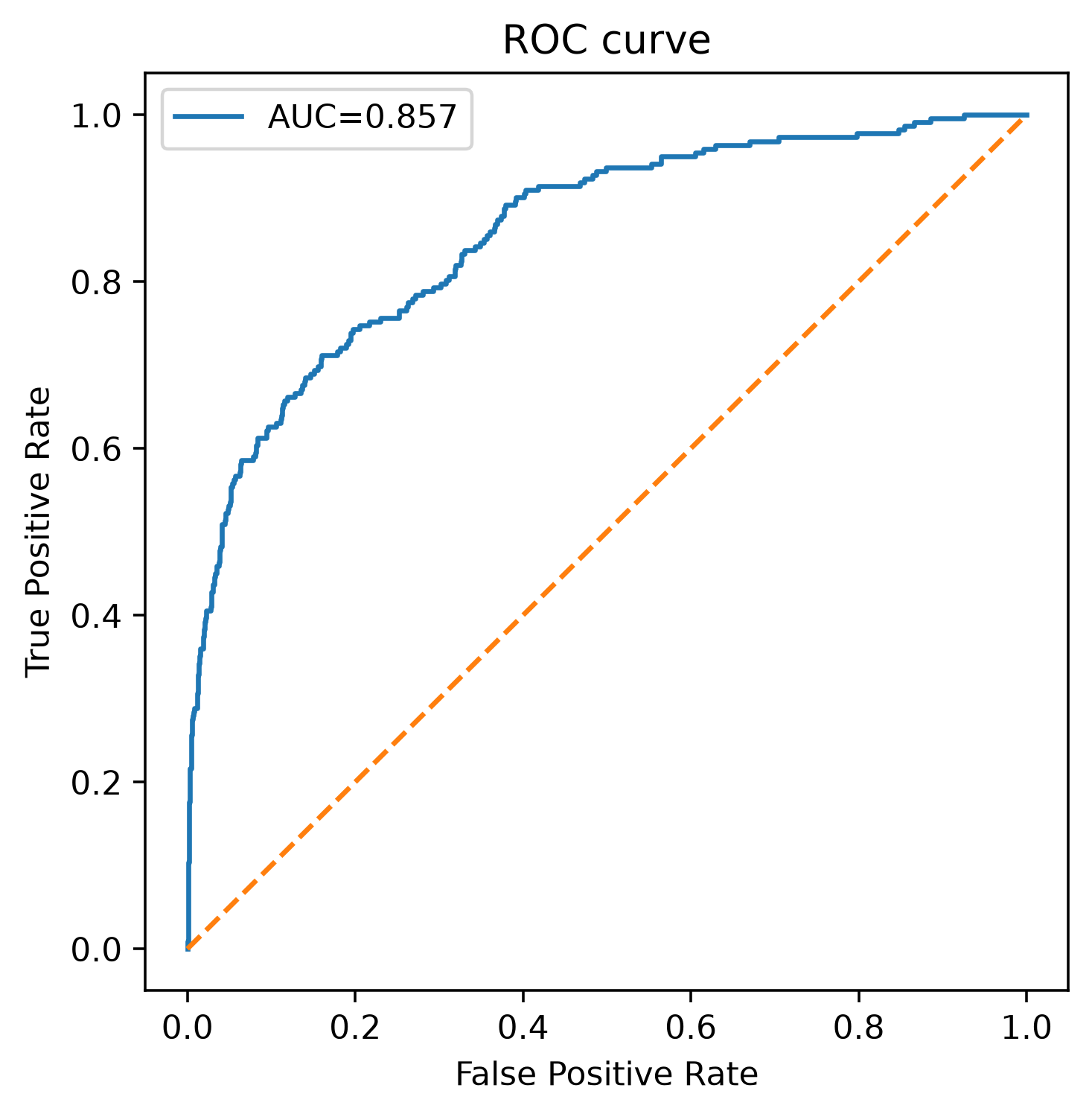
9. ROC Curve and ROC-AUC
ROC plots
TPR \quad \text{vs.}\quad FPR
over thresholds.
AUC measures ranking discrimination: how well positives tend to receive higher scores than negatives.
Show the code
from sklearn.metrics import roc_curve,roc_auc_scorefpr,tpr,_=roc_curve(y_test,prob)auc=roc_auc_score(y_test,prob)fig,ax=plt.subplots(figsize=(5,5))ax.plot(fpr,tpr,label=f"AUC={auc:.3f}")ax.plot([0,1],[0,1],linestyle="--")ax.set(xlabel="False Positive Rate",ylabel="True Positive Rate", title="ROC curve")ax.legend()plt.show()
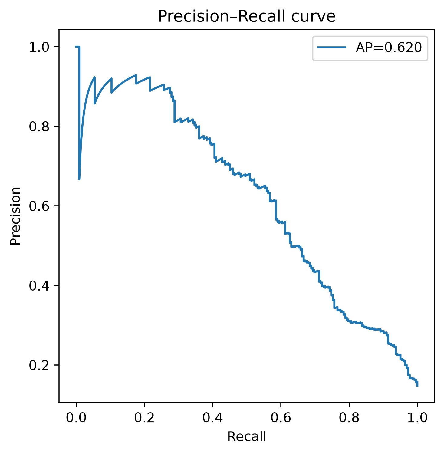
10. Precision–Recall Curve
For rare positive classes, PR curves often expose the useful operating region more directly.
Show the code
from sklearn.metrics import precision_recall_curve,average_precision_scoreprecision,recall,_=precision_recall_curve(y_test,prob)ap=average_precision_score(y_test,prob)fig,ax=plt.subplots(figsize=(5,5))ax.plot(recall,precision,label=f"AP={ap:.3f}")ax.set(xlabel="Recall",ylabel="Precision",title="Precision–Recall curve")ax.legend()plt.show()
11. Log Loss — Reward Honest Probabilities
For binary classification:
-\frac1n\sum_i
[y_i\log p_i+(1-y_i)\log(1-p_i)].
Confident wrong predictions are punished strongly.
Use when probability quality matters, not merely hard labels.
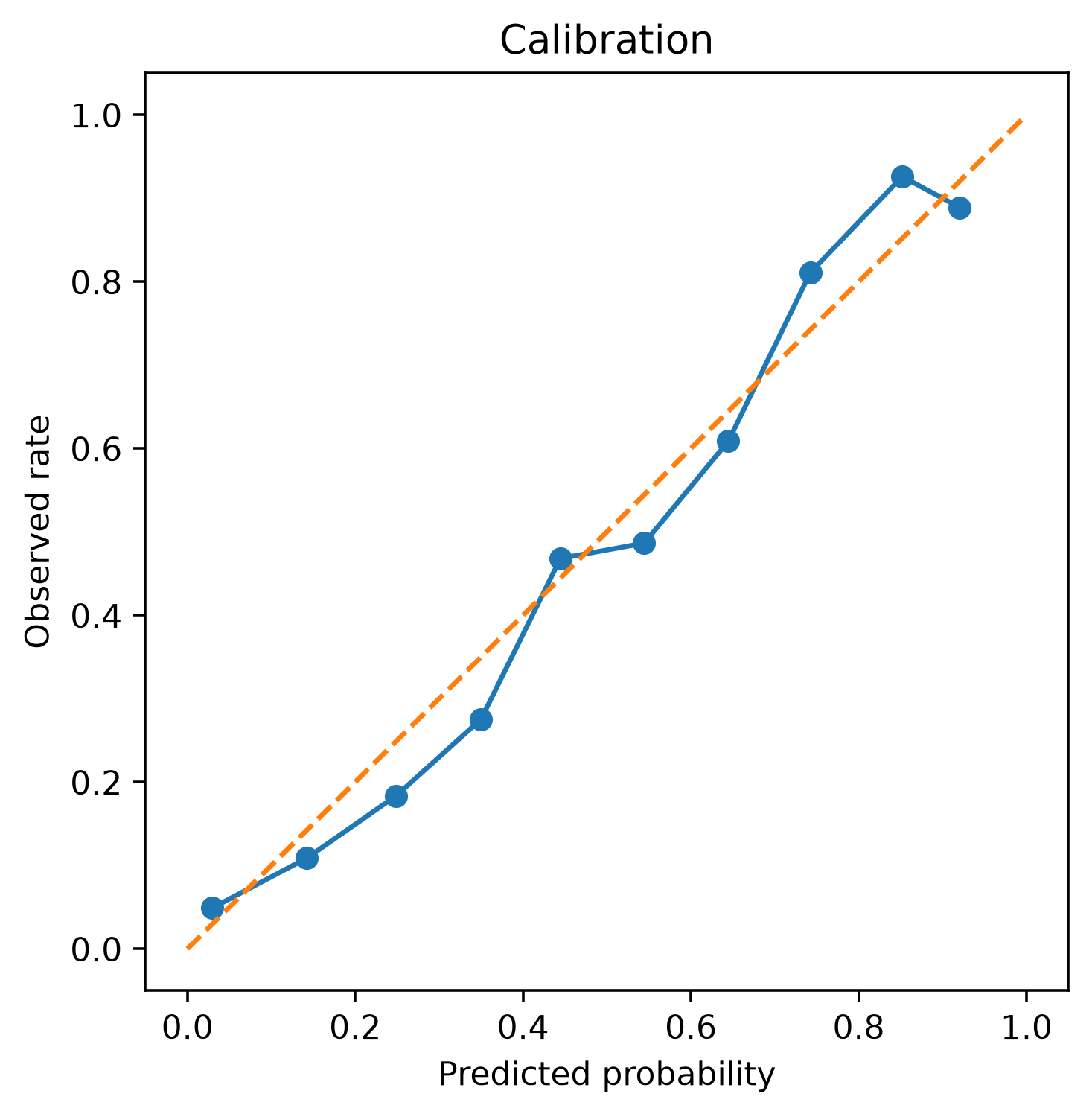
12. Calibration — Does 0.8 Mean About 80%?
A calibrated model satisfies approximately:
P(Y=1\mid \hat p\approx0.8)\approx0.8.
Show the code
from sklearn.calibration import calibration_curveobs,pred=calibration_curve(y_test,prob,n_bins=10)fig,ax=plt.subplots(figsize=(5,5))ax.plot(pred,obs,marker="o")ax.plot([0,1],[0,1],linestyle="--")ax.set(xlabel="Predicted probability",ylabel="Observed rate", title="Calibration")plt.show()
Ranking and calibration are separate properties.
13. Regression Metrics
Suppose residuals are
e_i=y_i-\hat y_i.
MAE
MAE=\frac1n\sum|e_i|.
Easy to interpret in target units and less dominated by large errors than MSE.
from sklearn.model_selection import cross_validatescores=cross_validate( LogisticRegression(max_iter=1000), X,y, cv=5, scoring=["roc_auc","average_precision","neg_log_loss"])pd.DataFrame(scores).filter(like="test_").describe()
test_roc_auc
test_average_precision
test_neg_log_loss
count
5.000000
5.000000
5.000000
mean
0.880999
0.646018
-0.271305
std
0.008790
0.029056
0.010784
min
0.872216
0.614416
-0.282189
25%
0.872343
0.630749
-0.280157
50%
0.881902
0.632345
-0.274053
75%
0.886150
0.668374
-0.262065
max
0.892385
0.684208
-0.258062
Report variation, not only the mean.
17. Choose the Split That Matches Reality
IID rows
Random K-fold may be appropriate.
Imbalanced classification
Use stratification.
Multiple rows per person/device/account
Use grouped splitting to prevent entity leakage.
Future prediction
Use time-ordered validation.
The split is part of the model
A sophisticated metric on an unrealistic split produces a sophisticated-looking wrong answer.
18. Interactive Cross-Validation Variability
Show repeated split simulation
from sklearn.model_selection import StratifiedKFold,cross_val_scorevals=[]for seed inrange(15): cv=StratifiedKFold(n_splits=5,shuffle=True,random_state=seed) s=cross_val_score( LogisticRegression(max_iter=1000), X,y,cv=cv,scoring="roc_auc" ) vals += [{"seed":seed,"fold":i+1,"auc":v} for i,v inenumerate(s)]cv_df=pd.DataFrame(vals)
Show the code
fig=px.scatter(cv_df,x="seed",y="auc",color="fold", title="Performance varies across validation samples")fig.show()
19. Hyperparameter Tuning Without Cheating
Hyperparameters are selected using training/validation information.
Examples:
regularization strength,
tree depth,
number of trees,
learning rate,
neighborhood size.
Tools include:
grid search,
randomized search,
successive halving,
Bayesian/optimization frameworks such as Optuna.
Never tune repeatedly on the final test set.
20. Learning Curves — More Data or Better Model?
Plot training and validation performance against training-set size.
Interpretation:
train high, validation low
→ overfitting / variance problem

both low
→ underfitting / bias or weak features

validation still improving with n
→ more data may help
21. Validation Curves — What Does Complexity Do?
Vary one hyperparameter and compare train vs validation scores.
Example: tree depth.
depth too small → underfit
depth moderate  → useful region
depth huge      → training perfect, validation deteriorates
22. Confidence Intervals and Bootstrap
A metric is an estimate from a finite sample.
Bootstrap evaluation:
test rows
  ↓ sample with replacement
metric₁

repeat B times
  ↓
distribution of metric
  ↓
uncertainty interval