Machine Learning Algorithms: A Practical Map of How Models Learn

Understand the recurring mathematical ideas behind modern ML algorithms, when to use each family, and how their behavior changes through interactive simulations.

🧠 Do not memorize 30 algorithms. Learn the few ideas that keep reappearing.

Most machine-learning algorithms repeatedly use some combination of similarity, linear combination, probability, partitioning, optimization, averaging, sequential error correction and representation learning.

1. Start with the Learning Problem

Given observations

\mathcal D=\{(x_i,y_i)\}_{i=1}^{n},

supervised learning seeks a function

\hat f:X\rightarrow Y

that performs well on unseen observations.

DATA → REPRESENTATION → ALGORITHM → PARAMETERS → PREDICTION → LOSS → LEARNING

TipVocabulary worth owning

feature · target · parameter · hyperparameter · loss · regularization · decision boundary · bias · variance · generalization

2. The Algorithm Family Map

📏 Linear models

Learn weighted combinations.

Linear regression · Logistic regression · Ridge · Lasso

🌳 Trees

Learn recursive decision rules.

Decision tree · Random forest · Gradient boosting

📍 Similarity

Nearby observations influence each other.

kNN · kernels · clustering

📐 Margins

Find separating boundaries.

SVM

🎲 Probabilistic

Model uncertainty/distributions.

Naive Bayes · probabilistic models

🧩 Unsupervised

Discover structure without labels.

k-means · PCA · anomaly detection

🧠 Neural

Compose learned nonlinear representations.

MLP · CNN · Transformer-style representations

3. Linear Regression — Learn a Weighted Sum

\hat y=\beta_0+\beta_1x_1+\cdots+\beta_px_p

Ordinary least squares minimizes

\text{MSE}=\frac1n\sum_{i=1}^{n}(y_i-\hat y_i)^2.

import numpy as np, pandas as pd
import matplotlib.pyplot as plt

rng=np.random.default_rng(4)
x=rng.uniform(0,10,120)
y=18+7*x+rng.normal(0,8,len(x))

from sklearn.linear_model import LinearRegression

X=x.reshape(-1,1)
model=LinearRegression().fit(X,y)

fig,ax=plt.subplots(figsize=(7,4))
ax.scatter(x,y,alpha=.45)
order=np.argsort(x)
ax.plot(x[order],model.predict(X)[order],linewidth=2)
ax.set(title="Linear regression: learn the best weighted line",
       xlabel="Advertising spend",ylabel="Sales")
plt.show()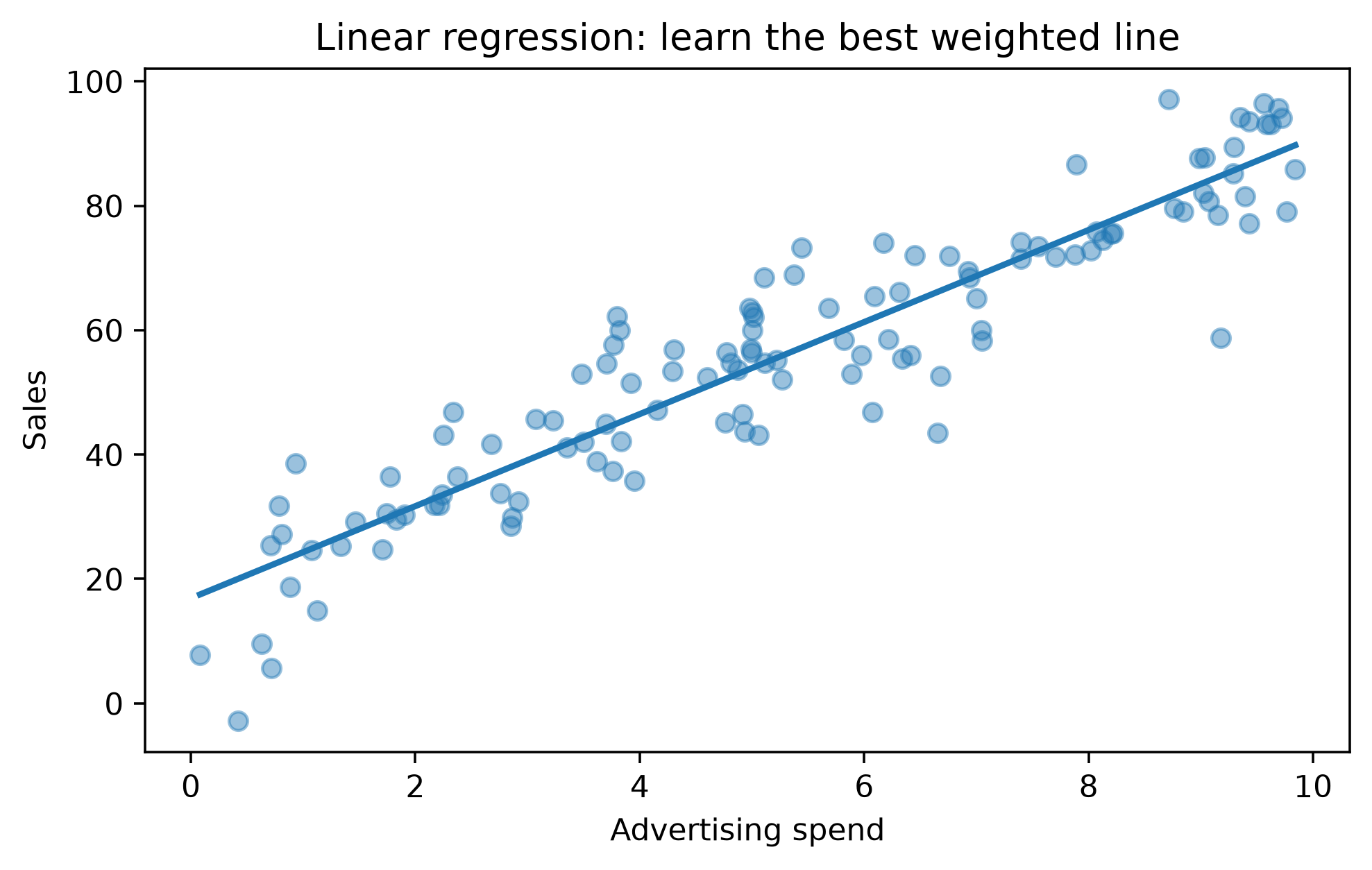

Use when

• relationship is approximately additive,
• interpretability matters,
• you need a strong baseline,
• extrapolation has defensible meaning.

4. Gradient Descent — The Recurring Optimization Idea

Many algorithms learn parameters by moving downhill on a loss:

\theta_{t+1}=\theta_t-\eta\nabla_\theta L(\theta_t).

η is the learning rate.

viewof lr = Inputs.range([0.01, 1.05], {value:0.18, step:0.01, label:"Learning rate η"})
viewof steps = Inputs.range([1, 30], {value:10, step:1, label:"Gradient steps"})

loss = x => (x-3)**2 + 1
path = {
  let w=-4, a=[{step:0,w,loss:loss(w)}];
  for(let i=1;i<=steps;i++){
    let grad=2*(w-3);
    w=w-lr*grad;
    a.push({step:i,w,loss:loss(w)});
  }
  return a
}
Plot.plot({
  height:330,
  x:{label:"parameter θ"}, y:{label:"loss"},
  marks:[
    Plot.line(d3.range(-5,8,.05).map(x=>({x,y:loss(x)})),{x:"x",y:"y"}),
    Plot.dot(path,{x:"w",y:"loss",fill:"step",r:5,tip:true})
  ]
})

Recurring idea

Gradient descent appears far beyond linear regression: logistic models, neural networks and many differentiable learning systems repeatedly optimize a loss by following gradients.

5. Logistic Regression — Linear Scores Become Probabilities

z=\beta_0+\beta^Tx

P(Y=1\mid x)=\sigma(z)=\frac{1}{1+e^{-z}}.

The model is linear in log-odds, not probability.

from sklearn.datasets import make_classification
from sklearn.linear_model import LogisticRegression

Xc,yc=make_classification(
    n_samples=700,n_features=2,n_redundant=0,
    n_clusters_per_class=1,class_sep=1.15,random_state=7
)
clf=LogisticRegression().fit(Xc,yc)

Use logistic regression as a highly valuable classification baseline—especially when calibrated probabilities and coefficient interpretation matter.

6. k-Nearest Neighbors — Learn by Similarity

For classification:

\hat y(x)=\operatorname{mode}\{y_i:i\in N_k(x)\}.

The central question becomes:

What does nearby mean?

viewof kval = Inputs.range([1,31], {value:5,step:2,label:"Neighbors k"})

from sklearn.neighbors import KNeighborsClassifier
knn=KNeighborsClassifier(n_neighbors=5).fit(Xc,yc)

Important lesson

kNN exposes why feature scaling matters. If salary ranges into hundreds of thousands while another feature ranges from 0–1, Euclidean distance can become mostly “salary distance.”

7. Decision Trees — Learn If/Then Regions

A tree repeatedly asks questions such as:

support_tickets > 3?
        /        \
      yes        no
     /            \
tenure < 6?     low risk

For classification, splits commonly reduce impurity. Gini impurity is

G=1-\sum_{k=1}^{K}p_k^2.

from sklearn.tree import DecisionTreeClassifier, plot_tree

tree=DecisionTreeClassifier(max_depth=3,random_state=2).fit(Xc,yc)
fig,ax=plt.subplots(figsize=(10,5))
plot_tree(tree,filled=True,ax=ax)
plt.show()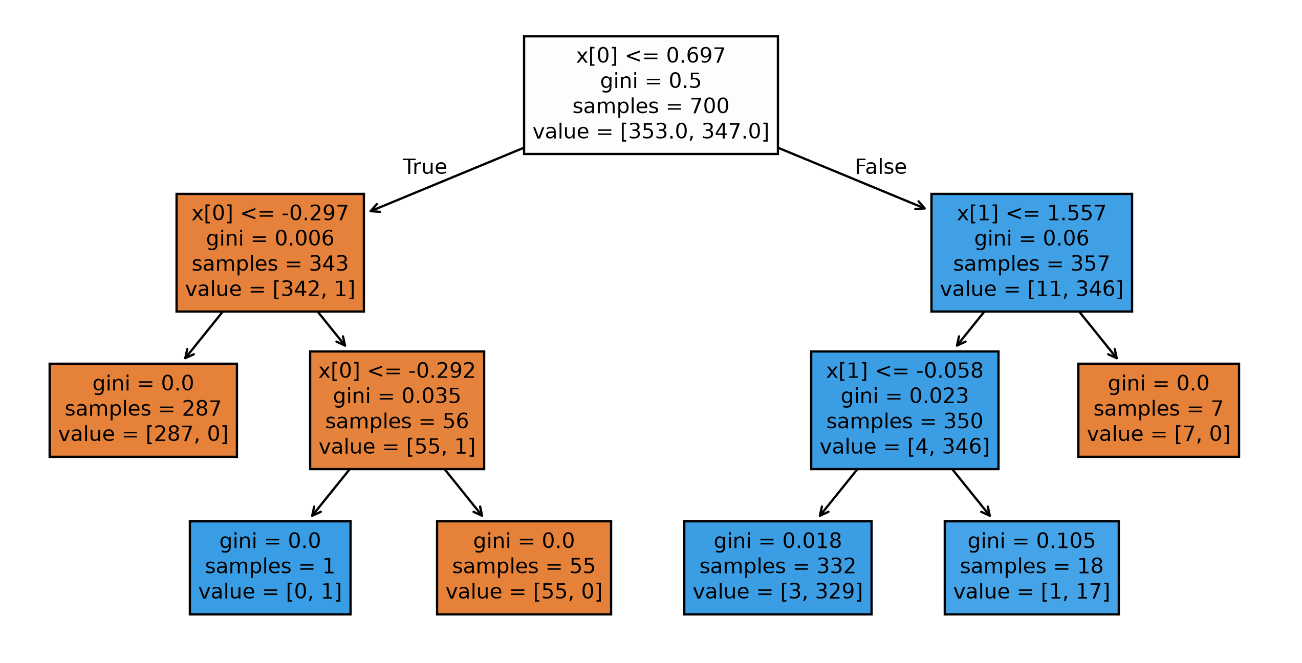

Trees naturally learn:

• thresholds,
• nonlinearities,
• interactions.

But a deep tree can memorize training data.

8. Random Forest — Many Unstable Trees Become Stable

A random forest trains many randomized trees and aggregates predictions:

\hat f(x)=\frac1B\sum_{b=1}^{B}\hat f_b(x)

for regression, with voting/probability averaging for classification.

The recurring idea is variance reduction through averaging.

from sklearn.ensemble import RandomForestClassifier

rf=RandomForestClassifier(
    n_estimators=300,
    max_features="sqrt",
    random_state=42
)
rf.fit(X_train,y_train)

9. Gradient Boosting — Learn from Previous Errors

Boosting builds an additive model:

F_M(x)=F_0(x)+\sum_{m=1}^{M}\eta h_m(x).

Each new learner is chosen to improve what the current ensemble gets wrong.

Bagging vs boosting

Random forest / bagging: build many diverse learners largely independently → average.

Boosting: build learners sequentially → each corrects the current ensemble.

Common modern tabular implementations include gradient-boosted trees such as XGBoost, LightGBM and CatBoost.

10. Support Vector Machines — Maximize the Margin

For a linear separator:

w^Tx+b=0.

SVMs seek a boundary with a large margin, with regularization controlling the tradeoff between margin and violations.

Kernel methods allow nonlinear boundaries through similarity in an implicit feature space.

Good conceptual lesson:

The training points nearest the boundary can matter much more than distant points.

11. Naive Bayes — Turn Bayes’ Rule into a Classifier

P(y\mid x_1,\dots,x_p) \propto P(y)\prod_jP(x_j\mid y).

The conditional-independence assumption is “naive,” yet the method can be surprisingly effective, especially for sparse text/count features.

12. k-Means — Find Centers Without Labels

k-means minimizes within-cluster squared distance:

\sum_{k=1}^{K}\sum_{x_i\in C_k}\|x_i-\mu_k\|^2.

from sklearn.datasets import make_blobs
from sklearn.cluster import KMeans

Xu,_=make_blobs(n_samples=700,centers=4,cluster_std=.8,random_state=12)
km=KMeans(n_clusters=4,n_init="auto",random_state=12).fit(Xu)

fig,ax=plt.subplots(figsize=(6,5))
ax.scatter(Xu[:,0],Xu[:,1],c=km.labels_,alpha=.45)
ax.scatter(km.cluster_centers_[:,0],km.cluster_centers_[:,1],
           marker="X",s=180)
ax.set_title("k-means: discover geometric groups")
plt.show()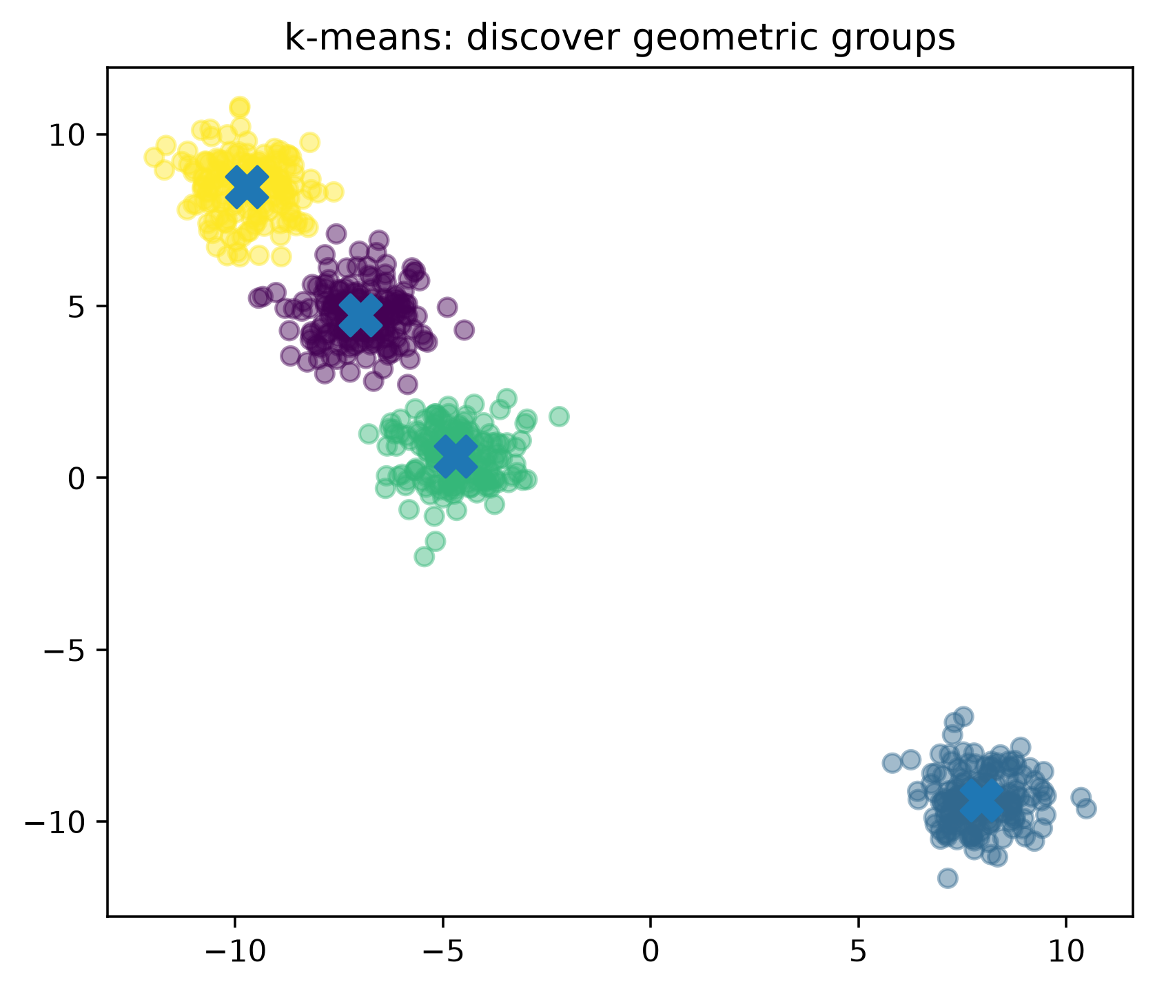

Clusters are mathematical groupings—not automatically real customer personas.

13. PCA — Rotate Toward Important Variation

PCA creates orthogonal directions maximizing variance.

For centered X, principal directions come from eigenvectors of its covariance matrix or equivalently an SVD.

z_1=w_1^Tx.

Use for:

• compression,
• visualization,
• denoising,
• decorrelation,
• understanding high-dimensional structure.

Do not automatically assume “largest variance = most predictive.”

14. Neural Networks — Compose Representations

A neuron computes

h=\phi(w^Tx+b).

Layers compose these operations:

x\rightarrow h_1\rightarrow h_2\rightarrow\cdots\rightarrow\hat y.

The major conceptual difference is that neural networks can learn representations and predictors jointly.

15. Regularization — Control Complexity

Ridge:

L_{\text{ridge}}=L+\lambda\sum_j\beta_j^2.

Lasso:

L_{\text{lasso}}=L+\lambda\sum_j|\beta_j|.

Regularization encodes the preference:

Fit the data—but not with arbitrary complexity.

This idea recurs in linear models, trees, boosting and neural networks under different names and mechanisms.

16. Bias–Variance: Why Algorithms Behave Differently

Expected prediction error can be understood conceptually as

\text{Error}\approx \text{Bias}^2+\text{Variance}+\text{Irreducible Noise}.

• shallow tree → potentially high bias,
• unconstrained deep tree → potentially high variance,
• random forest → reduces variance by averaging,
• boosting → often reduces bias while controlling complexity.

17. Practical Algorithm Choice

Situation	Strong starting points
Interpretable regression	Linear/Ridge
Interpretable classification	Logistic regression
Tabular nonlinear data	Gradient boosting / Random forest
Strong simple baseline	Linear/logistic + tree ensemble
Sparse text baseline	Logistic regression / Naive Bayes
Local similarity matters	kNN
Unlabeled grouping	k-means
Dimensional compression	PCA
Images/audio/text at scale	neural representation models

Do not choose by leaderboard folklore

Start with the data structure, target, sample size, constraints, interpretability, latency and validation design. Then compare credible baselines empirically.

18. The Algorithm Learning Ladder

LINEARITY → PROBABILITY → DISTANCE → TREES → ENSEMBLES → UNSUPERVISED STRUCTURE → REPRESENTATION LEARNING

Summary

The recurring ideas matter more than memorizing model names:

• weighted combinations,
• probability,
• similarity,
• recursive partitioning,
• optimization,
• regularization,
• averaging,
• sequential error correction,
• latent representation.

When you meet a new algorithm, ask:

What does it optimize? What representation does it assume? How does it control complexity? What kinds of structure can it express?